<< 返回本书主页
<< Back to the afterword page

8 流行性

吕汶桧 Wenhui Lyu

Jan. 2022

codes

8.1 背景问题

不同事物的流行程度存在差别。流行性往往呈现为幂律分布：受关注少的事物远多于受关注多的事物，有同样关注量的事物的数量总和在全体中的占比（$y$$y$），是其关注量（$x$$x$）的幂函数，亦即

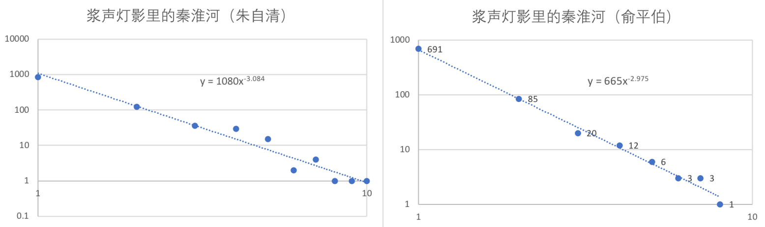
一个例子是文本中的词语出现次数

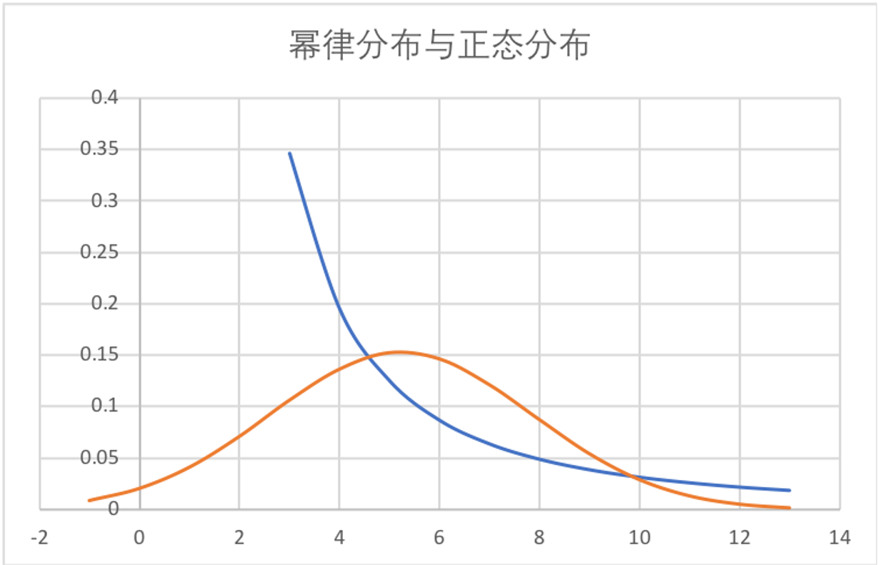
与正态分布相比，幂律分布是“偏态”的（不平等）。它有如下几个特点：

• 较小取值者有很大的占比；
• “中等收入群体”不够大；
• 较大取值者的占比也不是极低，“总有几个富人”。亦即“长尾”（long tail）性质，$\underset{x\to \mathrm{\infty }}{lim}{\displaystyle \frac{x+y}{x}}=1$$\lim_{x\to\infty}\dfrac{x+y}{x}=1$。

此外，幂律还是无标度（scale-free）、自相似的（self-similar），$F(ax)=bF(x)$$F(ax)=bF(x)$。

关注程度－数量的幂律分布，经过几步数学变换，就可以变成排位序－关注程度的分布。

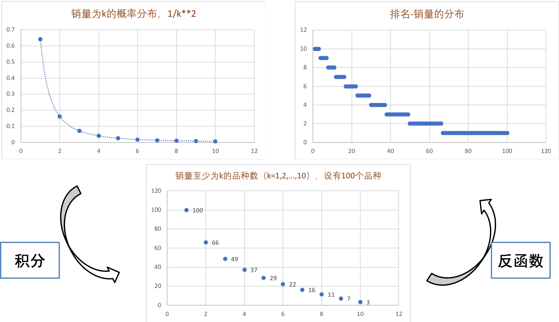
排位序－关注程度的分布也呈幂律分布。位次越高的事物，越受欢迎。这一定律由齐普夫首先发现，故被称为齐普夫律（Zipf's law）。他发现，在《尤利西斯》中，把词语按照出现频次$f$$f$由高到低排序，每一词语的位次为$r$$r$（$r=1$$r=1$为出现次数最多的词语），有如下规律存在：

其中$A$$A$为常数。后来的补充性研究做了进一步的厘正：

排位序－关注程度的分布让我们发现，生活中某些常常谈及的东西，和学术研究的某些经典成果，也来自幂律分布的性质，例如

• 2/8律：前20%的人/事物占有80%的关注。
• “长尾下的小生意”：排位序－关注程度的分布也有长尾性质，这意味着，排位不高的事物，受关注度的总和依然可以很大。亦即，对于$\mathrm{\forall }k$$\forall k$，只要$max$$max$足够大，${\int }_k^{max}{\displaystyle \frac{a}{x}}dx$$\int_{k}^{max}\dfrac{a}{x}dx$依然可以很大。Amazon、淘宝做的就是“长尾下的小生意”。

以上，我们讨论了流行性问题的现象、性质和规律。而流行性问题的成因或机理是什么呢？一个重要的理论是“富者愈富”：正因为人们喜欢追捧本来就很受欢迎的事物，事物的受欢迎程度才呈幂律分布。

在作业中，我们就要来模拟“富者愈富”的过程，看看最终是否会得到幂律分布的结果。

8.2 计算实践：富者愈富过程的模拟

codes

8.2.1 作业描述与算法思路

按照顺序创建一系列网页：$1,2,3,\dots ,j,\dots ,n=10000$$1,2,3,\ldots,j,\ldots,n=10000$

当创建网页$j$$j$时，以概率$p$$p$或$1-p$$1-p$选择$a$$a$或$b$$b$执行：

• $a$$a$. 以概率$p$$p$，均匀地、随机地选择一个早先创建的网页$i$$i$，建立一个从$j$$j$到$i$$i$的链接
• $b$$b$. 以$1-p$$1-p$的概率，按照与已有入度成正比的概率，选择一个早先创建的网页$i$$i$，建立一个从$j$$j$到$i$$i$的链接。

分别取$p=0.25,0.75$$p=0.25,0.75$运行程序。分析结果，观察最后的结果是否符合幂律分布。

节点入度	$0$$0$	$1$$1$	$2$$2$	$3$$3$	$4$$4$	$\dots$$\ldots$	$m$$m$
节点个数	$n_0$$n_0$	$n_1$$n_1$	$n_2$$n_2$	$n_3$$n_3$	$n_4$$n_4$	$\dots$$\ldots$	$n_m$$n_m$

本次作业有一个特别要求：尽量不用太大的存储空间。如果我们在每一步创建下一个网页时，都要记住前面所有网页分别链接到了哪个网页，运行到后面总网页数较大时，就会占用很大的存储空间，运行速度会比较慢。

事实上，我们只用在每一步记住不同频数的网页有多少个，列表的长度最多为$m$$m$，这远小于$n$$n$。因为我们不用明确地知道当前创建的网页$j$$j$链接到了之前的哪个网页$i$$i$上，而只需要知道$j$$j$链接到了入度为何（设为$f$$f$）的网页上，然后对入度－个数的表格进行操作（$n_f$$n_f$减小$1$$1$，$n_{f+1}$$n_{f+1}$增加$1$$1$），具体可见我代码中的degreeDictModifier函数。

此外，只存储节点入度－节点个数的信息时，如何实现随机选择一个网页，如何与入度成正比选择一个网页？我用到了random库的choices方法，采用了不同的加权值，实现了两种选择方式。具体可见我代码中的webCreate函数。

8.2.2 编程实现与要点说明

首先，定义一个函数degreeDictModifier，用以更新节点入度－节点个数的信息（被存储在“入度字典”degreeDict里）：输入原先的入度字典degreeDict和被选中网页的入度choice，返回更新后的入度字典degreeDict。

xxxxxxxxxx
1
1
def degreeDictModifier(degreeDict, choice): 

入度为choice的网页数减小$1$$1$：

xxxxxxxxxx
1
1
    degreeDict[choice] -= 1

入度为choice + 1的网页数增加$1$$1$：

xxxxxxxxxx
6
1
    designated = choice + 1
2
    if designated in degreeDict.keys():
3
        degreeDict[designated] += 1
4
    else:
5
        degreeDict[designated] = 1
6
    return degreeDict

接着，定义函数webCreate，创建新网页，并将其链接到之前创建的一个网页，调用degreeDictModifier函数，对degreeDict做出更新。

xxxxxxxxxx
3
1
def webCreate(degreeDict, p):
2
    degreeKinds = list(degreeDict.keys()) # 现有网页有的度数一共有这么些种
3
    degreeCount = list(degreeDict.values()) # 每一元素表示，度数为某一种的网页一共有几个

调用random库生成一个$[0,1]$$[0,1]$的随机数，它小于$p$$p$的概率为$p$$p$，大于$p$$p$的概率为$1-p$$1-p$。

• 以概率$p$$p$随机选择一个网页链接。我调用了random库的choices方法。对于每一种节点入度，按照这一入度共有多少网页进行加权weights=degreeCount，这样，选择某一入度的网页的概率与这一入度的总网页数成正比，而选择某一个网页的概率是相等的。

xxxxxxxxxx
5
1
    randNum = random.random()
2
    if randNum < p:
3
        randChoiceList = random.choices(degreeKinds, weights=degreeCount, k=1) 
4
        randChoice = randChoiceList[0]
5
        degreeDict = degreeDictModifier(degreeDict, randChoice)

• 以概率$1-p$$1-p$与入度成正比选择一个网页。对于某一入度kind，计算这一入度的网页数cnt和该入度的乘积（cnt * kind），存储在newWeights里，用这一数据给每一入度的网页加权。这样加权后，某一个网页被选中的概率与其入度成正比。

xxxxxxxxxx
9
1
    else:
2
        newWeights = []
3
        for kind, cnt in degreeDict.items():
4
            newWeights.append(cnt * kind)
5
        slantedChoiceList = random.choices(degreeKinds, weights=newWeights, k=1)
6
        slantedChoice = slantedChoiceList[0]
7
        degreeDict = degreeDictModifier(degreeDict, slantedChoice)
8
    degreeDict[0] += 1
9
    return degreeDict

定义函数webCreateSeries，循环调用webCreate，完成$10000$$10000$个网页的创建，并把最终的degreeDict输出到结果文件output.csv中，返回作图需要的数据。

xxxxxxxxxx
4
1
def webCreateSeries(n, p, outputF):
2
    print('* * * * * * A new round begins. n = %i, p = %.2f * * * * * *' % (n, p))
3
    cnt = 0
4
    outputF.write('n = %i p = %.2f\n' % (n, p))

循环完成10000个网页的创建，得到最终的degreeDict：

xxxxxxxxxx
9
1
    degreeDict = {0:1}
2
    while True:
3
        cnt += 1
4
        if cnt >= n:
5
            break
6
        if cnt % 100 == 0:
7
            print('%i pages have been created.' % cnt, end = '\r')
8
        degreeDict = webCreate(degreeDict, p)
9
    print()

输出最终的degreeDict到output.csv：

xxxxxxxxxx
15
1
    degreeList = list(degreeDict.items())
2
    degreeList.sort(key = lambda x:x[0])
3
    ## 删除网页数为0的度数，不然csv里一行太长了不好看
4
    for i in range(degreeList[0][0], degreeList[-1][0] + 1):
5
        if degreeDict[i] == 0:
6
            del degreeDict[i]
7
    degreeKinds = degreeDict.keys() 
8
    degreeCount = degreeDict.values() 
9
    outputF.write('degree,')
10
    for degreeKind in degreeKinds:
11
        outputF.write('%i,' % degreeKind)
12
    outputF.write('\namount,')
13
    for degreeCNT in degreeCount:
14
        outputF.write('%i,' % degreeCNT)
15
    outputF.write('\n')

整理数据，以方便主程序中作图，返回作图需要的数据xPoints, yPoints。

xxxxxxxxxx
16
1
    # 为了画图，补上网页数为0的度数
2
    degreeList = list(degreeDict.items())
3
    degreeList.sort(key = lambda x:x[0])
4
    for i in range(degreeList[0][0], degreeList[-1][0] + 1):
5
        if i not in degreeDict.keys():
6
            degreeDict[i] = 0 # for log scale
7
        elif degreeDict[i] == 0:
8
            degreeDict[i] == 0 # for log scale
9
    degreeList = list(degreeDict.items())
10
    degreeList.sort(key = lambda x:x[0])
11
    degreeKinds = [degreeList[i][0] for i in range(len(degreeList))]
12
    degreeCount = [degreeList[i][1] for i in range(len(degreeList))]
13
    xPoints = np.array(degreeKinds)
14
    yPoints = np.array(degreeCount)
15
    print('This round all done.')
16
    return xPoints, yPoints

主程序就比较简单了，直接给定n、p值调用webCreateSeries即可，得到相应的横轴纵轴数据x1, y1和x2, y2。

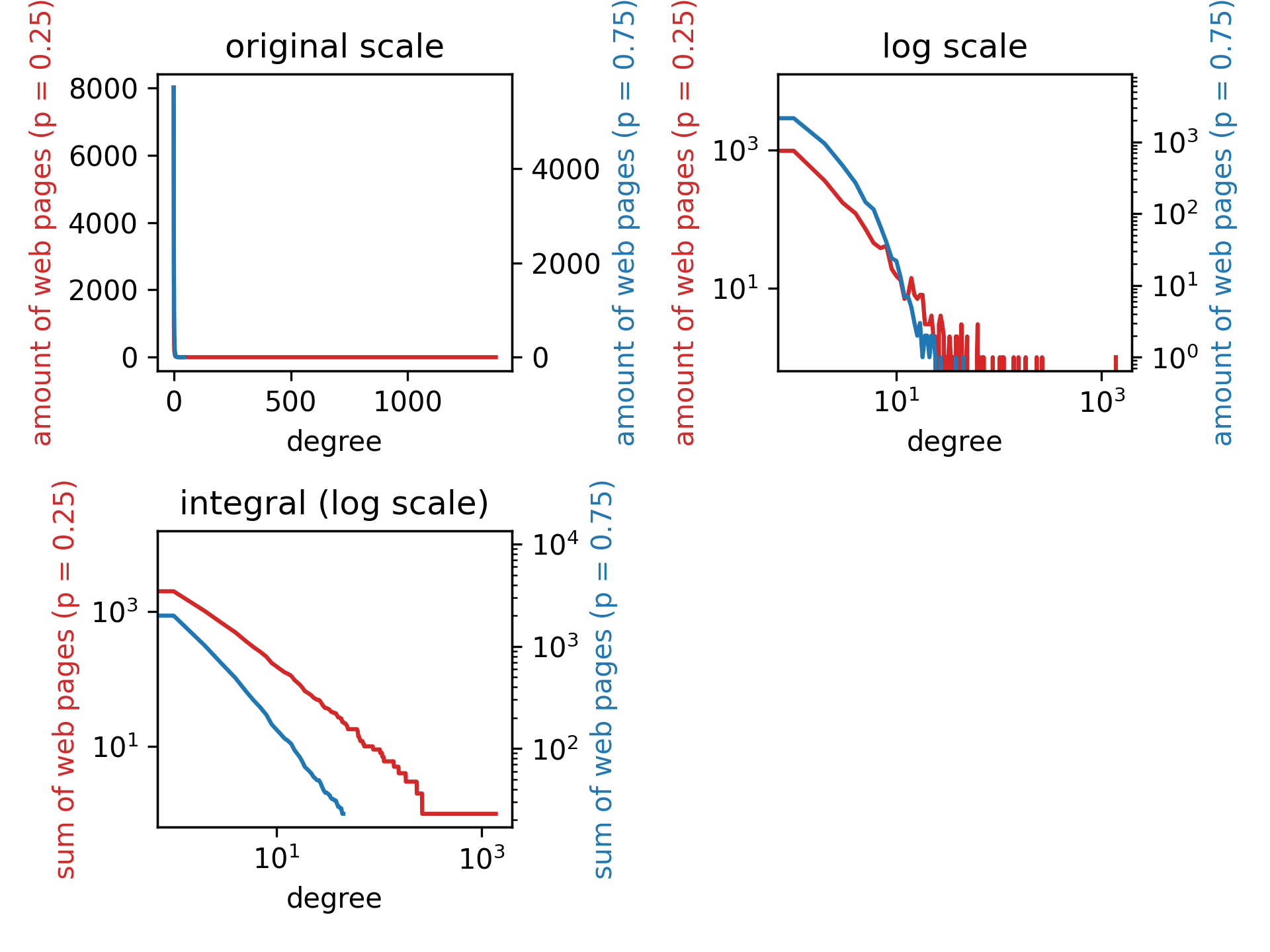
xxxxxxxxxx
10
1
outputF = open('output.csv', 'w')
2
fig = plt.figure()
3
ax1 = plt.subplot(2,2,1)
4
ax3 = plt.subplot(2,2,2)
5
ax5 = plt.subplot(2,2,3)
6
# n = 10000, p = 0.25
7
x1, y1 = webCreateSeries(10000, 0.25, outputF)
8
# n = 10000, p = 0.75
9
x2, y2 = webCreateSeries(10000, 0.75, outputF)
10
outputF.close()

接下来就是作图。先作入度－个数图（ax1和ax2）。该图应当符合幂律分布。

xxxxxxxxxx
13
1
## original scale
2
print('Drawing the picture...')
3
color1 = 'tab:red'
4
ax1.set_title('original scale')
5
ax1.plot(x1,y1,color=color1)
6
ax1.set_xlabel('degree')
7
ax1.set_ylabel('amount of web pages (p = 0.25)',color=color1)
8
ax1.tick_params(axis='y')
9
ax2 = ax1.twinx() # 把两次的结果画进同一个坐标系
10
color2 = 'tab:blue'
11
ax2.plot(x2,y2,color=color2)
12
ax2.set_ylabel('amount of web pages (p = 0.75)',color=color2)
13
ax2.tick_params(axis='y')

对入度和幂律取双对数作图（ax3和ax4）。该图应当是一条直线。

xxxxxxxxxx
13
1
ax3.set_title('log scale')
2
ax3.plot(x1,y1,color=color1)
3
ax3.set_xlabel('degree')
4
ax3.set_ylabel('amount of web pages (p = 0.25)',color=color1)
5
ax3.tick_params(axis='y')
6
ax3.set_xscale('log')
7
ax3.set_yscale('log')
8
ax4 = ax3.twinx() 
9
ax4.plot(x2,y2,color=color2)
10
ax4.set_ylabel('amount of web pages (p = 0.75)',color=color2)
11
ax4.tick_params(axis='y')
12
ax4.set_xscale('log')
13
ax4.set_yscale('log')

取双对数作图后，入度较大时，图形呈锯齿状，有的入度恰好存在网页，有的入度不存在网页。为了让图更好看，让网页数$amount(degree)$$amount(degree)$对$degree$$degree$在$[degre{e}_i,degre{e}_{max}]$$[degree_i,degree_{max}]$积分，$w={\int }_{degre{e}_i}^{degre{e}_{max}}amount(degree)$$w=\int_{degree_i}^{degree_{max}}amount(degree)$，它指的是有多少网页的入度大于$degre{e}_i$$degree_i$。

得到入度－大于该入度的总网页数$w$$w$后，取双对数作图ax5和ax6。分析$w$$w$的表达式，这一图形应为一条直线。

xxxxxxxxxx
25
1
ax5.set_title('integral (log scale)')
2
y1_new = np.copy(y1)
3
for i in range(len(x1)):
4
    pageSum1 = np.sum(y1[i:])
5
    y1_new[i] = pageSum1
6
y2_new = np.copy(y2)
7
for i in range(len(x2)):
8
    pageSum2 = np.sum(y1[i:])
9
    y2_new[i] = pageSum2
10
ax5.plot(x1,y1_new,color=color1)
11
ax5.set_xlabel('degree')
12
ax5.set_ylabel('sum of web pages (p = 0.25)',color=color1)
13
ax5.tick_params(axis='y')
14
ax5.set_xscale('log')
15
ax5.set_yscale('log')
16
ax6 = ax5.twinx()
17
ax6.plot(x2,y2_new,color=color2)
18
ax6.set_ylabel('sum of web pages (p = 0.75)',color=color2)
19
ax6.tick_params(axis='y')
20
ax6.set_xscale('log')
21
ax6.set_yscale('log')
22

23
fig.tight_layout()
24
plt.show()
25
fig.savefig('output.png', dpi=300)

8.2.3 结果与分析

n = 10000 p = 0.25		n = 10000 p = 0.25		n = 10000 p = 0.75
degree	amount	degree	amount	degree	amount
0	8005	31	1	0	5714
1	973	32	1	1	2136
2	360	33	2	2	948
3	172	34	1	3	467
4	121	36	1	4	269
5	72	38	2	5	145
6	45	39	2	6	115
7	38	41	1	7	66
8	41	43	3	8	40
9	19	45	1	9	24
10	15	47	1	10	22
11	13	48	1	11	13
12	7	49	2	12	7
13	8	61	1	13	7
14	14	62	3	14	5
15	8	64	1	15	3
16	7	65	1	16	2
17	8	69	1	17	3
18	8	71	1	18	1
19	3	87	1	19	2
20	3	102	1	20	2
21	3	107	1	21	1
22	4	111	1	22	2
23	2	139	1	23	2
24	2	155	1	24	1
26	3	182	1	27	1
27	4	233	1	38	1
28	3	263	1	45	1
29	2	1376	1

 

在我们的算法产生完$10000$$10000$个网页后，“入度 — 网页数”基本上呈幂律分布。这一点在左下图中体现得尤为明显。取双对数做图后，“入度 — 大于这一入度的网页总数”的图像基本是一条直线。

接下来分析p值对于这一分布的影响。通过比较$n=10000,p=0.25$$n = 10000, p = 0.25$与$n=10000,p=0.75$$n = 10000, p = 0.75$的输出结果，$p$$p$的值对于最后的分布很可能有以下影响（是否真的有这些影响，还需要更严格的数学证明，或取更多组数据做统计学分析）：

• $p$$p$越小，最受欢迎的网页的入度（$m$$m$）越大，较受欢迎的网页（例如入度$\ge 10$$\geq10$）的总数越大。这是因为，$p$$p$越小，创建某一网页时选择“跟风”路径的概率更高，即以与入度成正比的概率链接到网页。网页已有入度越高，越容易被链接到，富者越富。最终状态里，富人也会更多。
• $p$$p$越小，无人问津的网页越多，$p=0.25$$p=0.25$时有8005个，$p=0.75$$p=0.75$时有5714个。（这在图中没有表示出来，第一张图两条线叠在一起了，第二张图里入度为$0$$0$的点没法取对数。）这是因为，$p$$p$越小，创建某一网页时选择“平均主义”的概率越低，一开始就无人问津的网页更难被链接到，从而逐渐累积起来。

<< 返回本书主页
<< Back to the afterword page