<< 返回本书主页
<< Back to the afterword page

1 社会网络基础

吕汶桧 Wenhui Lyu

Jan. 2022

codes

1.1 背景问题

“网络”由节点组成，节点之间可能有边相连。网络常常是对社会的一种有效抽象，节点代表社会中的行动者，边代表行动者之间的联系。

我们可以用一个矩阵（称为邻接矩阵）来表示网络，在程序中一般就是对应一个二维数组。邻接矩阵在$(i,j)$$(i,j)$的值，表示$i$$i$与$j$$j$之间边的权重。一种基本的情形是权重为$0$$0$或$1$$1$，$0$$0$表示有边，$1$$1$表示没有边，此时的网络也称为“图”。例如，

这个矩阵就表示如下一个网络（或图），节点符号A，B，C，D，分别对应矩阵的第1，2，3，4行和列。

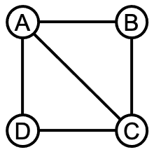
一个节点与自己总是没有边的，因此，矩阵从左上到右下的对角线上都是$0$$0$。对于一个无向图，邻接矩阵$A(i,j)=A(j,i)$$A(i,j)=A(j,i)$，亦即这一矩阵是对称的，以从左上到右下的对角线为轴。

基于图的邻接矩阵，我们可以通过计算得到对应社会网络的一些结构信息。例如，把一行内的值相加，就可以得到，该行对应的人有多少朋友。另一个例子是矩阵的乘幂，例如$A^2(i,j)$$A^2(i,j)$表示节点$i$$i$和$j$$j$之间的长度为$2$$2$的路径一共有多少条，也可以解释为$i$$i$和$j$$j$的共同朋友的个数。

利用这些计算操作，我们可以对网络的性质做出分析，这可以用以检验和社会网络相关的理论假设。作业“聚集系数和嵌入性”就是网络分析的一个例子。另一个作业则检验了社会网络学说的一个理论假设，即“友谊悖论”。

1.2 计算实践

1.2.1 聚集系数与嵌入性

codes

1.2.1.1 作业描述与算法思路

本次作业的主要任务是计算某一社会网络中，每个节点的聚集系数，以及每条边的嵌入性。

在一个网络中，不同人的社交密度或强度（intensity）不一样，有的人把自己的朋友聚集起来的能力很强——ta的朋友往往互相之间也认识。我们用“聚集系数”来刻画这一现象。节点$i$$i$的聚集系数指的是，$i$$i$的朋友们中，两两之间也是朋友的概率。

计算聚集系数的基本思路如下：我先分析邻接矩阵，用一个字典变量friend_dict存储“谁是谁的朋友”，字典的键（key）i指的是节点$i\in [0,n)$$i\in[0,n)$，节点$i$$i$的朋友$j,k,\dots \in [0,n)$$j,k,\ldots\in[0,n)$被存储在该键对应的值（value）里（值是一个列表）。接着，我再两两分析节点$i$$i$的朋友（我把他们俩称为以节点$i$$i$为中介的“间接朋友”），用friend_dict存储的信息验证，他们俩是否为“直接朋友”。节点$i$$i$的聚集系数就是“直接朋友”和“间接朋友”的比值。

两个人之间的关系也有性质上的差别，有的关系深深嵌入了周围的社交圈中——不仅他们俩是朋友关系，而且他们俩的共同好友很多。我们用“嵌入性”来刻画这一现象。边$(i,j)$$(i,j)$的嵌入性，指的是节点$i$$i$与$j$$j$的共同朋友数。

计算嵌入性时，我一一分析网络中的边。对于边$(i,j)$$(i,j)$，我检查，节点$i$$i$的朋友有多少也是节点$j$$j$的朋友，这一过程也是用friend_dict完成的。

1.2.1.2 编程实现与要点说明

首先，我们读取样本数据文件，把文件里的矩阵数据存储在一个numpy 2d-array A里。

28
1
import numpy as np
2

3
def arrayGen(filename):
4
    f = open(filename, 'r')
5
    r_list = f.readlines()
6
    f.close()
7
    A = []
8
    for line in r_list:
9
        if line == '\n':
10
            continue
11
        line = line.strip('\n')
12
        line = line.strip()
13
        row_list = line.split()
14
        for k in range(len(row_list)):
15
            row_list[k] = row_list[k].strip()
16
            row_list[k] = int(row_list[k])
17
        A.append(row_list)
18
    n = len(A[0])
19
    print('输入矩阵路径：%s' % filename)
20
    A = np.array(A)
21
    return A, n
22

23
try:
24
    filename = input('请输入邻接矩阵文件名（如net3.txt）：')
25
    A, n = arrayGen('./input/%s' % filename)
26
except:
27
    print('输入错误，使用默认文件net3.txt。')
28
    A, n = arrayGen('./input/net3.txt')

分析这一网络，我们把“谁是谁的朋友”存储在一个字典变量friend_dict里，字典的键（key）$N\in [0,n)$$N\in[0,n)$是节点，节点$i\in [0,n)$$i\in[0,n)$的朋友被存储在该键对应的值（value）里。

6
1
friend_dict = {}
2
for i in range(n):
3
    friend_dict[i] = []
4
    for j in range(n):
5
        if A[i][j] == 1:
6
            friend_dict[i].append(j)

接着，我再两两分析节点$i$$i$的朋友（他们俩是“间接朋友”，以节点$i$$i$为中介），用friend_dict存储的信息验证，他们俩是否为“直接朋友”。以节点$i$$i$为中介的间接朋友数存储在变量PossTriCl里，这些人中的直接朋友数存储在变量TriCl里。聚集系数$ClCo={\displaystyle \frac{TriCl}{PossTriCl}}$$ClCo=\dfrac{TriCl}{PossTriCl}$。每一节点的聚集系数被存储在一个字典变量ClCo_dict里。

15
1
ClCo_dict = {} # ClCo表示clustering coefficient
2
for (person, friend_list) in friend_dict.items():
3
    TriCl = 0
4
    for x in range(len(friend_list)):
5
        friend1 = friend_list[x]
6
        for y in range(x+1, len(friend_list)):
7
            friend2 = friend_list[y]
8
            if A[friend1][friend2] == 1:
9
                TriCl += 1
10
    PossTriCl = len(friend_list) * (len(friend_list) - 1) / 2
11
    if PossTriCl == 0:
12
        ClCo = 0
13
    else:
14
        ClCo = TriCl / PossTriCl
15
    ClCo_dict[person] = ClCo

最后，我们在控制台里打印出各节点聚集系数的情况。

10
1
print()
2
print('clustering coefficient as following:')
3
ClCo_list = list(ClCo_dict.items())
4
ClCo_list.sort(key = lambda x:x[1], reverse = True)
5
if len(ClCo_dict) < 10:
6
    for item in ClCo_list:
7
        print('node', str(item[0]) + ':', '%.2f' % item[1])
8
else:
9
    for item in ClCo_list[0:10]:
10
        print('node', str(item[0]) + ':', '%.2f' % item[1])

控制台输出的一个例子如下（由于样本数据较大，仅输出聚集系数排名前十的节点）。

14
1
>>> 请输入邻接矩阵文件名（如net3.txt）：net3.txt
2
>>> 输入矩阵路径：./input/net3.txt
3
>>> 
4
>>> clustering coefficient as following:
5
>>> node 16: 1.00
6
>>> node 34: 1.00
7
>>> node 23: 0.67
8
>>> node 29: 0.67
9
>>> node 1: 0.50
10
>>> node 8: 0.50
11
>>> node 22: 0.50
12
>>> node 27: 0.50
13
>>> node 31: 0.50
14
>>> node 36: 0.50

接着计算网络中各边的嵌入性。利用friend_dict遍历所有边、计算两个人的共同朋友数。

8
1
embd_dict = {}
2
for (person, friend_list) in friend_dict.items():
3
    for friend_a in friend_list:
4
        if friend_a > person:
5
            embd_dict[person, friend_a] = 0
6
            for friend_b in friend_dict[friend_a]:
7
                if friend_b in friend_list:
8
                    embd_dict[person, friend_a] += 1

输出结果到控制台。

14
1
print()
2
print('embeddedness as following:')
3
embd_list = list(embd_dict.items())
4
embd_list.sort(key = lambda x:x[1], reverse = True)
5
if len(embd_list) < 10:
6
    for item in embd_list:
7
        print('edge', end = ' ')
8
        print(item[0], end = '')
9
        print(':', str(item[1]))
10
else:
11
    for item in embd_list[0:10]:
12
        print('edge', end = ' ')
13
        print(item[0], end = '')
14
        print(':', str(item[1]))

由于样本数据较大，仅输出嵌入性排名前十的边。

11
1
>>> embeddedness as following:
2
>>> edge (2, 13): 4
3
>>> edge (0, 10): 3
4
>>> edge (2, 25): 3
5
>>> edge (2, 31): 3
6
>>> edge (4, 10): 3
7
>>> edge (13, 25): 3
8
>>> edge (13, 31): 3
9
>>> edge (0, 4): 2
10
>>> edge (0, 27): 2
11
>>> edge (1, 14): 2

1.2.2 友谊悖论的验证

codes

1.2.2.1 作业描述与算法思路

本次作业的主要任务是验证友谊悖论。这一悖论说的是，现实中多数人一般都感到朋友的朋友多于自己的朋友；尽管，直观上我们会觉得，既然有人觉得朋友的朋友多于自己的朋友，另一些人就会觉得朋友的朋友少于自己的朋友。

验证这一悖论，要在某个社会网络中进行。为了得到亟待验证的社会网络，一个方法当然是以现实生活的数据为基础、进行抽象和转化，我们在这次作业中采取的是另一个方法：基于“小世界”现象，生成一系列的网络。社会科学以“小世界”为主题的研究颇多，这些成果保证，我们生成的社会网络是对真实世界的合理模拟。

“小世界”现象指的是，邻接矩阵中任意两个点之间，都有一条很短的路径可以通达。之所以“小世界”现象存在，是因为社会网络有如下两个性质：

• 同质性（homophily）：一个圈子里的人往往互相都认识，网络中应当有很多三角形（参见第二讲三元闭包）。我们用初始规则度数$r$$r$模拟同质性，表示每一节点和编码相邻的节点之间的边数。这样，编码相近的节点之间会形成很多三角关系。
• 随机性（randomness）：除了小圈子以外，网络中还存在一些跨圈的边，这些边连接的两个节点没有共同朋友（没有形成三元闭包）。这些边的形成不是由于同处一个圈子，或多或少体现了随机性。是这些边保证了任意两点之间有一条很短的路径；否则，要连接不在同一圈子的节点时（例如，要把澳洲的一个庄园主和一个叙利亚难民连接起来），必须借助相邻节点之间的一条条规则边，甚至如此“翻山越岭”也不一定能连接起两个节点。我们用随机调整边占比$p$$p$来模拟随机性：按照初始规则度数生成的边中，比例为$p$$p$的边被删除， 同样数量的边随机地在任意两点间生成。

改变初始规则度数$r$$r$、随机调整边占比$p$$p$、总节点数$n$$n$，我们就可以得到一系列不同的社会网络。它们都有“小世界”现象，只是同质性、随机性和规模有所不同。对于每一网络，我们都检验友谊悖论是否成立。

为了检验某一网络是否存在友谊悖论，我一一检查网络中的每一节点。对于节点$i$$i$，如果他的朋友数（度数degree）比他朋友的平均度数小不少，那么节点$i$$i$就存在友谊悖论。如果节点$i$$i$度数刚好小于邻居的平均度数，节点$i$$i$很难明显感觉到朋友比自己更受欢迎。我具体设定的悖论觉知门槛是，节点$i$$i$度数的$1.1$$1.1$倍小于邻居的平均度数。对于整个网络，如果超过一半的节点都觉知到了友谊悖论，这一网络就存在友谊悖论。

1.2.2.2 编程实现与要点说明

首先，我们需要一个生成社会网络的函数neighbor_generator：输入总节点数n、初始规则度数r、随机调整边占比p，这个函数会输出一个表示社会网络的矩阵matr（numpy 2d-array）。

xxxxxxxxxx
3
1
def neighbor_generator(n, r, p):
2
    file = open('./output/generator_logs/{}'.format(time.strftime("%H:%M:%S")), 'w')
3
    matr = np.zeros((n,n))

初始规则边的建立：每一节点与相邻$r$$r$个节点建立规则边。当$n$$n$是偶数时，使节点$i$$i$与编码$\in [i+1,i+|\frac{r}{2}+1+r\mathrm{mod}2|]$$\in [i+1, i + |\frac{r}{2}+1+r \mod 2|]$的节点建立边即可；当$n$$n$是奇数时，执行同样的操作后，还需要删除$\frac{n-1}{2}$$\frac{n-1}{2}$条边。这样操作后，总边数为${\displaystyle \frac{n\times r}{2}}$$\dfrac{n \times r}{2}$。

xxxxxxxxxx
27
1
    file.write('Generating an orderly matrix with homophilous links...\n')
2
    edge_list = []
3
    for i in range(0,n):
4
        j_list = [(i + x) % n for x in range(1, int(r/2 + 1 + r % 2))]
5
        for j in j_list:
6
            matr[i][j] = 1
7
            matr[j][i] = 1
8
            if j > i:
9
                edge_list.append([i,j])
10
            else:
11
                edge_list.append([j,i])
12
    file.write('Writing the list of node pairs which do not have an edge...\n')
13
    empt_list = []
14
    for i in range(0,n):
15
        if i % 100 == 0:
16
            file.write('%i nodes processed...' % i)
17
        for j in range(i+1,n):
18
            if matr[i][j] == 0:
19
                empt_list.append([i,j])
20
    file.write('For now, number of edges in Matrix A: %i\n' % np.sum(matr))
21
    if r % 2 != 0: 
22
        for i in range(0, n-1, 2):
23
            matr[i][i+1] = 0
24
            matr[i+1][i] = 0
25
            edge_list.remove([i, i + 1])
26
            empt_list.append([i, i + 1])
27
    file.write('Number of edges in Matrix A: %i\n' % np.sum(matr))

随机调整边：对于已建立的规则边（存储在exc_edge中），比例为p的边被删除，并随机在无关系的两个节点之间（存储在exc_empt中）生成新边。

xxxxxxxxxx
9
1
    file.write('Introducing randomness...\n')
2
    exc_edge = random.sample(edge_list, int(n * r * p / 2))
3
    exc_empt = random.sample(empt_list, int(n * r * p / 2))
4
    for item in exc_edge:
5
        matr[item[0]][item[1]] = 0
6
        matr[item[1]][item[0]] = 0
7
    for item in exc_empt:
8
        matr[item[0]][item[1]] = 1
9
        matr[item[1]][item[0]] = 1

输出矩阵

xxxxxxxxxx
2
1
  np.savetxt('./output/generator_logs/neighbor_original_{}'.format(time.strftime("%H:%M:%S")),matr,fmt='%i')
2
    return matr

除此之外，我们还需要一个验证友谊悖论的函数paradox：输入一个给定的矩阵，输出一个bool值，即它是否满足友谊悖论。

xxxxxxxxxx
1
1
def paradox(matr, n):

我先把“谁是谁的朋友”存储在字典变量fr_dict中，再用这个字典变量计算：节点$i$$i$的度数，存储在dg_dict[i]['self']；ta邻居的平均度数，存储在dg_dict[i]['nb']。

xxxxxxxxxx
20
1
    fr_dict = {}
2
    dg_dict = {}
3
    # generate fr_dict to store who's whose friend
4
    for i in range(0, n):
5
        fr_dict[i] = []
6
        for j in range(0, n):
7
            if matr[i][j] == 1:
8
                fr_dict[i].append(j)
9
    # generate the degrees of individuals
10
    for i in range(0, n):
11
        dg_dict[i] = {}
12
        dg_dict[i]['self'] = len(fr_dict[i])
13
    # generate the average degrees of neighbors
14
    for i in range(0, n):
15
        dg_dict[i]['nb'] = 0
16
        for friend in fr_dict[i]:
17
            if fr_dict[i] == []:
18
                dg_dict[i]['nb'] = 0
19
            else:
20
                dg_dict[i]['nb'] += dg_dict[friend]['self'] / len(fr_dict[i])

如果节点$i$$i$的度数的$1.1$$1.1$倍小于邻居的平均度数，ta就存在友谊悖论。如果网络中所有节点超过55%存在友谊悖论（pdScale > 0.55），这一网络就存在友谊悖论。

xxxxxxxxxx
6
1
    pdIndex = 0
2
    for i in range(0, n):
3
        if 1.1 * dg_dict[i]['self'] < dg_dict[i]['nb']:
4
            pdIndex += 1
5
    pdScale = pdIndex / n
6
    return [pdScale, pdScale > 0.5]

由于生成矩阵使用了随机数，随机过程的干扰可能导致单次生成的矩阵是一个特殊情况，对验证结论产生很大影响。因此，我们还需要一个计算友谊悖论期望值的函数pdE_calculator：输入一组特定的自变量（总节点数n、初始规则度数n、随机调整边占比n），运行矩阵生成函数一定次数loopCount，计算出现友谊悖论的节点比例pdScale的平均值，我们就得到该网络的友谊悖论期望值pdE。

xxxxxxxxxx
20
1
def pdE_calculator(n, r, p, loopCount = 100): # paradox expectation
2
    k = 0
3
    pdSum = 0
4
    while True:
5
        matr = neighbor_generator(n, r, p)
6
        pdScale = paradox(matr, n)[0]
7
        k += 1
8
        pdSum += pdScale
9
        if k == int(loopCount):
10
            print('given n = %i, r = %i, p = %.2f, the paradox scale has been successfully calculated' % (n, r, p), end = '\n') 
11
            break
12
        if n >= 500 or loopCount >= 300:
13
            if k == 1:
14
                print('wait a few seconds for the computer to process...', end ='\r')
15
            if n >= 500 and k % int(5000 / n) == 0 and k > 10:
16
                print('%i out of %i rounds have been successfully runned........' % (k, loopCount), end = '\r')
17
            if loopCount >= 300 and k % 100 == 0 and k > 300:
18
                print('%i out of %i rounds have been successfully runned........' % (k, loopCount), end = '\r')
19
    pdE = pdSum / loopCount
20
    return pdE

除此之外，我还定义了一个输出结果的函数pdOutput，便于反复调用。输入一组自变量值parameterList和对应的友谊悖论验证结果pdEList，它能在控制台打印结果、在csv文件中写入结果、使用matplotlib绘图。

xxxxxxxxxx
20
1
def pdOutput(parameter, parameterList, pdEList, f):
2
    print('Paradox scales of different %s values as following...' % parameter)
3
    f.write('%s,' % parameter)
4
    for i in parameterList:
5
        print(i, end = '\t')
6
        f.write(str(i) + ',')
7
    print()
8
    f.write('\nParadox Expectation,')
9
    for pd in pdEList:
10
        print('%.3f' % pd, end = '\t')
11
        f.write('%.3f' % pd + ',')
12
    print()
13
    f.write('\n')
14
    xPoints = np.array(parameterList)
15
    yPoints = np.array(pdEList)
16
    plotNumDict = {'n' : 1, 'r' : 2, 'p' : 3}
17
    plt.subplot(2, 2, plotNumDict[parameter])
18
    plt.plot(xPoints, yPoints, marker  = 'o')
19
    plt.xlabel('%s values' % parameter)
20
    plt.ylabel('average paradox scales')

以下是主程序

xxxxxxxxxx
5
1
import random
2
import os
3
import matplotlib.pyplot as plt
4
import numpy as np
5
import time

先准备好记录输出的csv文件。

xxxxxxxxxx
7
1
resultDir = './output'
2
if os.path.isdir(resultDir): 
3
    pass
4
else:
5
    os.makedirs(resultDir)
6
fname = './output/friendship paradox.csv'
7
f = open(fname, 'w')

我们先来验证，不同的网络规模$n$$n$对友谊悖论发生期望的影响。给定,$r=5,p=0.25$$r=5,p=0.25$，$n\in \{50,100,150,200,300,500,600,800,1000\}$$n\in\{50, 100, 150, 200, 300, 500, 600, 800, 1000\}$。对于每一个$n$$n$值，我们调用pdMean函数，设定loopCount为100，计算发生友谊悖论的比例，结果存储在n_pdList里。

xxxxxxxxxx
13
1
n_start = time.time()
2
print('*** Calculating paradox scales given different n values ***')
3
n_list = [50, 100, 150, 200, 300, 500, 600, 800, 1000] # more than 7 groups to make the tendency more explicit
4
n_pdList = []
5
for n in n_list:
6
    n_pdE = pdE_calculator(n = n, r = 5, p = 0.25)
7
    n_pdList.append(n_pdE)
8
pdOutput('n', n_list, n_pdList, f)
9
n_end = time.time()
10
n_span = n_end - n_start
11
n_time = '%i min %i s' % (n_span // 60, n_span % 60)
12
print('Paradox scales calculating of different n values cost', n_time)
13
print()

同理，我们再来验证，初始规则度数不同时，友谊悖论发生期望有何不同。给定$n=100,p=0.25$$n=100,p=0.25$，$r\in \{3,4,5,6,7,8,9,10\}$$r\in\{3, 4, 5, 6, 7, 8, 9, 10\}$，设定loopCount为100。

xxxxxxxxxx
12
1
print('*** Calculating paradox scales given different r values ***')
2
r_list = [3, 4, 5, 6, 7, 8, 9, 10]
3
r_pdList = []
4
for r in r_list:
5
    r_pdE = pdE_calculator(n = 100, r = r, p = 0.25)
6
    r_pdList.append(r_pdE)
7
pdOutput('r', r_list, r_pdList, f)
8
r_end = time.time()
9
r_span = r_end - n_end
10
r_time = '%i min %i s' % (r_span // 60, r_span % 60)
11
print('Paradox scales calculating of different r values cost', r_time)
12
print()

同理，我们最后来验证，随机调整边占比$p$$p$不同时，友谊悖论发生期望有何不同。给定$n=100,r=5$$n=100,r=5$，$p\in \{0.15,0.25,0.35,0.45,0.55,0.65,0.75,0.85,0.95\}$$p\in\{0.15, 0.25, 0.35, 0.45, 0.55, 0.65, 0.75, 0.85, 0.95\}$。

注意到，$p$$p$越大，随机数对矩阵生成的扰动就越大，我们需要增加循环数，亦即增加矩阵生成次数loopCount，保证友谊悖论节点比例的平均值能达致稳定。因此，我将循环数设为${\displaystyle \frac{75}{1-p}}$$\dfrac{75}{1-p}$。

xxxxxxxxxx
13
1
print('*** Calculating paradox scales given different p values ***')
2
p_list = [0.15, 0.25, 0.35, 0.45, 0.55, 0.65, 0.75, 0.85, 0.95]
3
p_pdList = []
4
for p in p_list:
5
    p_loop = 75 / (1 - p) 
6
    p_pdE = pdE_calculator(100, 5, p, p_loop)
7
    p_pdList.append(p_pdE)
8
pdOutput('p', p_list, p_pdList, f)
9
p_end = time.time()
10
p_span = p_end - r_end
11
p_time = '%i min %i s' % (p_span // 60, p_span % 60)
12
print('Paradox scales calculating of different p values cost', p_time)
13
print()

1.2.2.3 结果与分析

n	50	100	150	200	300	500	600	800	1000
Paradox Expectation	0.482	0.481	0.478	0.482	0.481	0.483	0.481	0.481	0.482
r	3	4	5	6	7	8	9	10
Paradox Expectation	0.547	0.511	0.486	0.465	0.451	0.429	0.406	0.4
p	0.15	0.25	0.35	0.45	0.55	0.65	0.75	0.85	0.95
Paradox Expectation	0.418	0.48	0.517	0.533	0.55	0.559	0.57	0.573	0.575

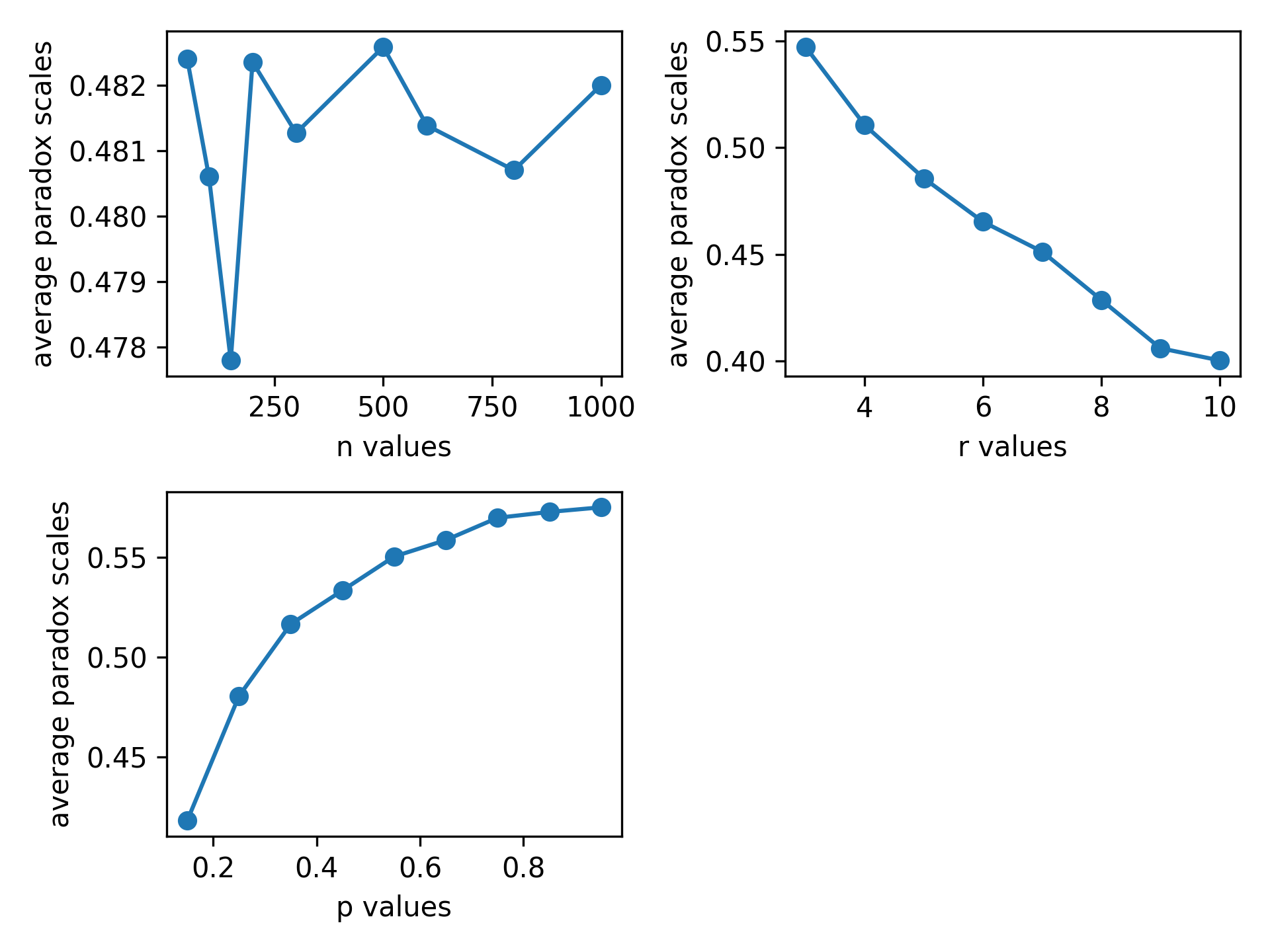
• 社会网络规模$n$$n$对友谊悖论节点比例平均值的影响不明朗。
• 随着初始规则度数$r$$r$变大，友谊悖论在全网络中的占比变小，友谊悖论更加弱。当$r\ge 5$$r\geq5$时，友谊悖论在全网络中的比例低于0.5，不再是一个社会普遍的现象。
• 随着随机调整边占比$p$$p$变大，友谊悖论在全网络中的占比变大，友谊悖论更加明显。当$p\ge 0.35$$p\geq0.35$时，友谊悖论在全网络中的比例高于0.5，可以说这时友谊悖论是一个普遍现象。

进一步的验证，还需要优化模型、增加取值、增加pdE_calculator()循环数loopCount后，进行严谨的统计学分析。我们的初步结论是，当$r$$r$较小、$p$$p$较大时，友谊悖论在全网络中的比例高于0.5，可以说这时友谊悖论是一个普遍现象。

<< 返回本书主页
<< Back to the afterword page